IP Packet Overhead
1 Introduction
What
does it cost for transport? This
question can be applied to moving goods and delivering services across
distances. King Hussein of
Let
me tell a true story about the first time I realized lower layer overhead
matters and makes a difference in performance results. The most compelling reason to understand the
overhead costs for transporting IP packets is the impact on performance. And performance becomes more important as more
voice, video, and data services use IP for content & service delivery. The world is going IP baby. IP over everything. These are the mantras of the Internet
Age. Adopt a common packet switched
& routed topology and global intercommunication is facilitated. Point to point dedicated connections are
replaced with multi-user networks that determine delivery on a per packet
basis. And that ties in to the story.
Once
upon a time I was a test engineer for a Tier 1 IP Service provider. There was a test process for evaluating the
performance of a POS (Packet over SONET) OC-48 interface on a high end backbone
router. As we will discuss later on,
OC-48 has a line rate of 2.488 Gbps. But after you remove the section, line, and
path overhead associated with SONET, 2.39616 Mbps of payload remains as useable
for transporting data (like PPP, HDLC, or Frame-Relay encapsulated IP
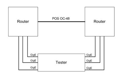
packets). To saturate the POS OC-48
link, the lab had an IP packet generator/analyzer (a packet blaster) with 6
Gigabit Ethernet test interfaces that linked into 6 GigE
interfaces on two routers interconnected with a POS OC-48 link. So there were three Gigabit Interfaces on
either side of the POS OC-48 allowing for up to three Gbps
of Ethernet IP packets to be sent across the POS link bidirectional. Refer to Figure I
for a graphic of the test topology.
Figure
I. POS OC-48
Test Topology
When
I ran the tests I had some of the oddest results I had ever encountered. Typically IP performance is a function of
packet distribution. The smaller the
size of the IP packets the more demanding routing them becomes to achieve the
same level of performance. A routing
engine has to dedicate the same processing lookup for a 40byte TCP SYN packet
as for a 1500 byte HTTP data packet but the 1500 byte packet carried a lot more
data with it. If there are increased
numbers of smaller packets are on a network, the more demanding it is for the
routers to perform at the same data rates.
Here is an example. Say the
network load is 15 Mbps (15,000,000 bits per second). To create that load using 1500 byte IP
packets using 802.3 100baseTX Ethernet, you would need to send 1219.116 packets
per second (we will discuss how we derived this rate later in the text). To create the same 15 Mbps condition using 40
byte IP packets (which with be transported over Ethernet using 64 byte Ethernet
Frames) would 22,321.429 packets per second.
That is more than 18 times as many packets to create the same bits on
the wire condition. So smaller packets
are more demanding than big packets.
They are shorter and often less latent, but their small size makes it
possible for there to be many more packets that need to be transported. And typically, the results reflect that and
fixed size tests using small packets tend to experience failure more often than
large size packet tests. But this test
yielded results that were counter-intuitive and the opposite of the expected
result. The tests were passing at 100%
utilization for 64 and 128 byte packet tests (controlled tests based on RFC
2544 that send fixed size packet tests using the sizes: 64, 128, 256, 512,
1024, 1280, and 1518), but dropping packets below line rate for larger
packets. So on
the face of it the router was doing better with massive volumes of smaller
packets while the bigger packets were causing problems. Another thing that should be pointed out is
that 100% line rate utilization equated to three Gbps
of IP Ethernet traffic. How could three Gbps of IP traffic traverse a link that has a maximum
payload capacity of 2.39616 Gbps? Every packet size should have experienced
loss at below line rate at rates consistent with the maximum capacity of the
OC-48 link. Three Gbps
is greater than 2.39616 Gbps. Except when it isn’t. What caused this anomaly? The answer was found in analyzing the
differences in lower layer overhead between Ethernet and POS.
As
this book will explain, a 46 byte IP packet inside of a 64 byte Ethernet frame
actually utilizes at least 84 bytes on the Ethernet wire. But only the 46 byte IP packet is routed onto
a POS link for transport. Now to
traverse the POS connection the 46 byte IP packet was encapsulated using HDLC
which places a 4 byte header on the packet plus a 2 byte checksum (it can also
use a 4 byte checksum but it was 2 bytes in this case) and a 1 byte flag to
delimit packets. So a 46 byte IP packet
on the POS link required 53 bytes to transport it in this scenario. So of the 84 bytes used on the Gigabit
Ethernet wire per 46 byte IP packet, only 53 bytes made it to the POS wire when
the IP packet was de-encapsulated and re-encapsulated using HDLC over
SONET. When you do the math and divide
53/84 only 63% of the load of the Gigabit Ethernet wire was translated to the POS
wire at this packet size. The result was
less than 2 Gbps of load was placed on the POS OC-48
from three Gigabit Ethernet links operating at 100% load. And that is less than the payload throughput
capability of OC-48 at 2.39616 Gbps. That is why the test succeeded. Because Ethernet is far from the most
efficient networking technology ever invented.
It is just one of the cheapest and easiest. Now the 128 byte packets tests created a
condition where the 148 bytes used on the Ethernet wire translated to 117 bytes
on the POS wire and 117/148 is closer to 79% of the traffic from the Ethernet
makes it to the POS, but that still creates 2.3716 Gbps
of load which is still less than the 2.3916 Gbps of
payload capacity OC-48 has available. As
the packet sizes get larger the fixed per packet overhead incurred by Ethernet
and the efficientcy of POS becomes less dramatic and
the three Gbps of Ethernet traffic is able to oversubscribe
the POS OC-48 and packet loss occurs because the interface is being asked to
transport more packets than is physically possible. That was the reason for the counter-intuitive
results. POS is more efficient than
Ethernet. And that is something that can
only be understood by analyzing physical and data-link overhead.
How
does anyone come into a situation where knowing the per packet layer1 &
layer2 overhead conditions for various technologies even matters you may
ask? The answer is found in IP test labs
all over the world. Anyone who has ever
used a packet blaster (a device that is designed to perform high end packet
generation and analysis) knows that the results are given in packet rates, not
bps. This is where calculating per
packet overhead including lower layer overhead comes into practical
application. Also, most test engineers
generate packets using IP Ethernet interfaces and often are testing interfaces
using a WAN technology (ATM, Frame-Relay, SONET, etc…). In that scenario it is key
to understand the differences between the IP packets on the interfaces you are
sending to and from, and the ones that are being traversed in the network
system under test.
1.1 Packets/Sec & Bits/Sec
IP
performance can be measured in a variety of ways. Packets per second (pps) is one
metric of network performance. So too is
bits per second (bps). Of course, bps is far more common in
marketing materials from service providers because it sounds impressive. One is reminded of the Doctor in Back to the
Future™ as he exclaimed ‘One point one
GIGAWATTS!!!’ as if that was more power than could be imagined (apologies to
the international audience and we will keep the American pop cultural references
to a minimum). So too is 10 Gbps. 10 billion
zeros and ones sent every second and processed by the receiver. That is a lot of zeros and ones to process
every second. It is impressive. But how many Ethernet Packets can be sent
over 10 Gbps.
What is the maximum number of packets that can be sent? Of course it is variable and a function of
the size of the packets. As one might
expect, smaller packets can achieve higher rates while bigger packets fill the
pipe more quickly. I am using 10 Gigabit
Ethernet as an example but the principles apply to every physical layer
technology discussed in this book.
How are pps and bps related? Well there is a mathematical equation that
allows anyone to calculate how many packets can be sent using a specified bps
and how many bits on the wire will be created by a given pps. Here is the equation:
pps x packet size (bytes) x 8
= bps
Now there
are some caveats and assumptions in this mathematical relationship. The number one key to this equation is that
all the packets have to be the same size for this equation to work. If the packet size is uniform the number of
packets can be multiplied by that size and multiplied by 8 to convert to bits
and will reflect a bit rate instead of a packet rate. Also the bps that is calculated reflect the number of bits on the wire that are in frames
(not all bits on the wire are always in frames). An additional equation multiplying the bits
that are not in frames per packet times the packet rate times 8 to convert to
bits. This can be considered layer 1
overhead bps and this can be added to the frame bps to reflect the total bits
on the wire.
The pps/bps equation will be referred to for each physical
layer medium discussed but there are subtle calculations that will modify it
for each technology.
1.2 OSI & TCP/IP Layer Models
Figure II.
OSI & TCP/IP Layer Models
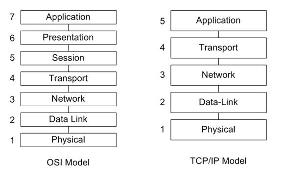
Both
of these models have logical similarities, and the main functional difference
is that the TCP/IP model aggregates layer 5,6, and 7 into
a single “Application’ layer. For the
purpose of this reference, the OSI model will be used as the model of choice
for reasons of familiarity. When people
refer to ‘Layer 7’ it is clear the model is the OSI model and the layer is the
‘Application’ layer. When you refer to
‘Layer 5’ the distinction is not as clear and not automatically assumed to be
the ‘Application’ layer. You know you
have arrived as an accepted model to describe the flow of data through a
network when there are jokes and rules of thumb that refer to your model. One of the ‘rules of thumb’ is ‘If you don’t have layer 1, you have
bupkis’ or something along that line. This is a way of saying physical layer is
paramount and often networking problems can be traced to the cables. One of the common jokes is references to
layers 8, 9, & 10 as being the economic, political, & religious layers
of networking. Economic factors play
into network decision making, politics can green light or 86 a project, and as
for religion, the reference is about zealot topics (MAC vs. Windows vs. Linux).
1.3
Organization
This
paper addresses how IP packets are encapsulated and transported using various common
Layer 1 & 2 technologies. The
chapters are designed to focus on a specific technology or set of standards and
describe how that technology applies itself to the transport of IP packets. Vendor implementations are very diverse and
sometimes may have capabilities beyond the standard feature set for a given
physical layer technology.
IEEE 802.3 Ethernet
– Clearly this chapter focuses on the transport of IP packets over standard
Ethernet networks, one of the world’s most popular networking technologies. People use CAT5 UTP with RJ-45 mod plugs
without even thinking about the operation of the interface they plug it into. This chapter covers the world’s most deployed
networking technology and how it is used to transport the world’s most popular
Layer 3 protocol. IP
over Ethernet.
ATM
– Don’t throw tomatoes. ATM is used to
send IP packets all the time. And to use
existing networks and SONET rings, ATM is established and continues to deliver
services reliably (most notably cell phone service).
Frame-Relay, PPP, &
HDLC – Frame-Relay networks are still found in
the deployed networks frequently and the encapsulation has similarities with
PPP & HDLC. The signaling is
completely different for each of these, but the encapsulations and overhead
incurred per packet are similar.
SONET and POS
– The world’s most popular long haul optical fiber technology
Chapter
8: Legacy Technologies, FDDI, ISDN, Token-Ring, X.25 – FDDI was one of the
first fiber technologies, ISDN is still used all over the world, Token-Ring is
primarily a LAN technology developed by IBM to compete with Ethernet, and X.25
was one of the first modern telecom technologies developed.
Chapter
9: Tunneling / Encryption, GRE, L2TP, MPLS, VLAN, IPSec, SSL
Chapter
10: Layer 3/4 Overhead, IP, IPv6, UDP, RTP, TCP
2 IEEE 802.3
Ethernet
Table
1.1 – Common Ethernet Speeds and Feeds
|
Name |
Connector |
Speed |
Distance |
|
10BASE-2 |
AUI |
10 Mbps |
500m |
|
10BASE-5 |
BNC |
10 Mbps |
200m |
|
10BASE-T |
RJ-45 |
10 Mbps |
100m |
|
100BASE-TX |
RJ-45 |
100 Mbps |
100m |
|
100BASE-FX |
ST, SC,
LC |
100 Mbps |
2000m |
|
1000BASE-T |
RJ-45 |
1 Gbps |
100m |
|
1000BASE-X |
ST, SC,
LC |
1 Gbps |
2000m |
|
10GBASE-X |
ST, SC,
LC |
10 Gbps |
2000m |
Ethernet
won. Ethernet interfaces are the number
one installed network interface on PCs, servers, and Unix Workstations. Ethernet has progressed from 10base2,
10base5, 10baseT with AUI, BNC, and RJ-45 connectors to 100baseTX and
100baseFX, 1000baseX, and 10000baseX.
For network administrators who supported BNC Ethernet networks, it is
easy to understand why they have been preempted by CAT5. For anyone who has not had the pleasure of
troubleshooting the ‘Christmas-light Topology’ that is a BNC Ethernet network,
the issue was that the network was a string of connected systems with 50Ω ohm terminators on each end. When there is an un-terminated break in the
string, the noise on the wire makes it impossible for any communication. So clever support technicians would carry
around a pocket of BNC T connectors so when the call came in that the
secretaries cannot print (an indication that the network is down), they would
validate the outage, and then ask who had moved offices to locate the most
likely source of the disconnect. The
likelihood was that the PC that was removed was taken with the BNC T connector
leaving two disconnected ends, and inserting a connector would resolve the
outage. CAT5 with RJ-45 modular
connectors links uses a star topology so if a station is disconnected from the
concentrator, hub, or switch, it only impacts that one station and none of the
others. That is a more fault tolerant
network architecture. That is why BNC
Ethernet LANs are not widely used anymore.
And it demonstrates how far Ethernet has come as a technology.
Now one thing that is interesting about IEEE 802.3
Ethernet is that the whether it is running over BNC, Fiber, at 10 Mbps, or 1 Gbps, the construction of the Ethernet frames is the
same. And while there are multiple
formats for the Ethernet header (802.2, 802.3, etc…), only Ethernet II is used to
encapsulate IP Packets. Refer to figure
1.1 for a graphic representation of the Ethernet II frame format. This is the format used to transport IP
packets over Ethernet networks.
Figure 1.1 – Ethernet II Frame Format
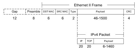
The numbers reflect the number of bytes used for
each field. Feel free to search the
Internet and most sites and standards documents will show this frame format
diagram for Ethernet II without the ‘Preamble’ and ‘IFG (Inter-Frame Gap)’
referred to. However these fields are
bits on the wire that exist between every Ethernet packet. The minimum Inter-frame gap is 96 bit times
and the preamble is 8 bytes. That is 12
bytes plus 8 bytes per frame that is on the wire at Layer 1, but not part of
the Ethernet frames. Every frame incurs
these bits and must have them to be transmitted, but they are not in the frames. So they don’t count. But they are counted as part of the 100
million bits per second sent by 100BASE-TX.
Also they are part of Gigabit Ethernet and 10 Gigabit Ethernet.
Here is a sample captured Ethernet II IP Packet
decoded. It is a Server to Client HTTP
200 OK packet.
Frame 1 (214 bytes on wire,
214 bytes captured)
Arrival Time:
Packet Length: 214 bytes
Capture Length: 214 bytes
Protocols in frame: eth:ip:tcp:http:data
Ethernet II, Src: fe:ff:
Destination: Xerox_00:
Source: fe:ff:
Type: IP (0x0800)
Internet Protocol,
Src: 216.239.59.99
(216.239.59.99), Dst:
145.254.160.237 (145.254.160.237)
Transmission Control
Protocol,
Hypertext Transfer Protocol
Data (160 bytes)
2.1
CSMA/CD
Carrier Sense Multiple Access Collision Detect is
the mechanism employed by IEEE 802.3 Ethernet interfaces to share a common
medium (like in wireless and half-duplex coax wire). Stations defer for a quiet period and then
start sending frames in bit serial form.
If a collision occurs, both stations backoff
and wait a random period before retrying.
In full-duplex mode, stations can send and receive without collisions as
there is a dedicated pipe per direction.
The CSMA/CD algorithms, collisions, and backoff
can impact Ethernet performance as well as per packet overhead. This is mainly seen in wireless 802.11x
(a/b/g/n) networks today as they are shared media and the access point or
infrastructure node that links to a wired network uses a half duplex mechanism
per radio channel. Some wireless vendors
employ proprietary implementations that associate and connect client radios
with infrastructure access points using two channels and then use one as the
‘upstream’ and one as ‘downstream’ to create a pseudo full-duplex mode of
operation. These implantations are not
covered under the 802.11x standards but they are used to improve the performance
of the wireless clients.
3 ATM
3.1
Asynchronous Transfer Mode
ATM will be around for decades. While other networking technologies may
provide more efficiency for IP Transport (there is a “cell tax” for using ATM for
transporting multiprotocol PDU’s
using ATM cells), ATM continues to be popular.
However, ATM continues to be a highly popular choice by telecommunication
companies and service providers because of the ability to provision Peak Cell
Rates (PCR) to specific Virtual Circuits (VCs) and provide bandwidth
guarantees. And for Voice and Video
Services, and specifically cell phones, the service quality of ATM makes up for
the cost of using it to transport IP packets.
In short, ATM continues to be the WAN technology
of choice for telecommunication companies looking to build out new service
areas. Now a major function of ATM
backbones is carrying IP packets. Having
worked for major telecommunications service providers, it was a commonly known
fact that IP transport represented 80% of the costs, but only 20% of the
revenues. ATM may only use 20% of the
bandwidth for Voice and Video, but as converse to the data, clearly that
portion would represent 80% of the revenues.
That is not to say ATM does not have engineering
and provisioning challenges that make IP backbones very tempting. Especially as IP services for Voice, Video,
and Data become more functional, fault tolerant, and usable, IP networks become
more practical and offer advantages. The
traditional issue with ATM networks is that VCs are unidirectional and for a
fully functional network, every ATM switch needs a VC to every other
switch. And often these switches are
configured with static VCs. This leads
to a provisioning nightmare as the number of network nodes grows. For each switch added to a network, the
number of VCs required to be configured equates to “N * (N-1)” VCs. Also, the VCs pointing at the new switch from
the other switches need to be added. This
approaches a tedious level of configuration and one mistake can leave a network
node disconnected from the network. And
a node failure is a major problem, especially if a node is acting as an interconnect. The
advantage of IP is dynamic routing protocols that allow routing to occur and
the network can ‘self-heal’ and find alternate paths to a destination if there
is one when a node fails.
And the biggest problem with IP Networks is the
default behavior of IP routers to use First-In,
First-Out (FIFO) queuing and, in the event of congestion, IP is best
effort. In other words, there is no
guaranteed delivery, and packets can be dropped. Often engineers fall back on the mechanisms of
higher layer protocols like TCP to resend dropped packets. If the sender does not receive an
acknowledgement packet (ACK), it resends the packet. Now this is fine for TCP based applications
like HTTP or email (SMTP). However,
Voice and Video are loss sensitive and resending lost frames does nothing to
make up for a gap in service (caused by lost packets). So Voice and Video and streaming media
typically use UDP and sometimes RTP for sending data. If Voice and Video frames are lost, service
quality degrades. So the challenges
facing IP deployments are how to deal with congestion and maintain service
quality for Voice and Video. Many
Service Providers deal with congestion by throwing bandwidth at the problem and
over-provisioning so there is no congestion.
New services like tunneling and MPLS seek to provide end-to-end service
quality and some of the advantages of ATM to the world of IP Networks. Part of this is to use different queuing
algorithms to preserve Voice and Video quality when congestion does occur. This is a real challenge when legacy IP
routing gear is considered and just one congested link using FIFO can trash
Voice and Video services. Period. So ATM
endures.
IP is growing and the ‘IP over everything’ mantra
will continue to gather momentum. But it
does not stand alone in the world of networking protocols.
ATM Signaling
Discussion of SVCs.
ATM cell header
VPI
– Virtual Path Identifier
VCI
– Virtual Channel Identifier
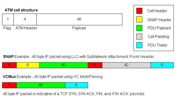
ATM Adaptation Layer 5 (AAL5)
AAL5
is the format ATM uses for sending IP packets.
ATM uses fixed size cells and IP packets are almost always bigger that
the 48 bytes available in a single cell.
So most IP packets require multiple cells to be
transported. And the process of
slicing the packets into cells and then reassembling them on the other side of
an ATM link is called, appropriately, Segmentation and Reassembly (SAR).
Figure 2.1
3.2
Case Study: ATM / Ethernet Comparison
The graph that was created in this case study was
designed to display the differences in bandwidth usage between Ethernet and
ATM. The blue and the pink data points
represent results from the same tests.
The pink display the bps load on the ATM interface, and the blue
represents the load on the GigEthernet interface in
the same test iterations. In this case,
the ATM AAL5 encapsulation used was VCMUX.
Here is an example of a real world test of an ATM
OC-3 being tested using GigEthernet ports to saturate
the interfaces:
Figure 2.2
Note that the ATM Interface usually is at or near
100% performance of the 149,760,000 bps that is it’s maximun capacity. So
the ATM load is usually in the high 148 Mbps to the low 149 Mbps range. Whereas the Ethernet load
ranges from 110 Mbps to 171 Mbps.
That is quite a sweeping difference.
And it has to do with how the IP packets are inserted into ATM cells
using the AAL5 PDUs described earlier. The packet sizes selected where designed to
hit the sweetest and the meanest spots for fitting packets in ATM Cells.
Take the example of the 106 byte and 107 byte IP Ethernet
packets (Refer to Table 2.2). A 106 byte
Ethernet packet will have the 18 byte IEEE Ethernet header removed when it
arrives at the networking device. That
leaves a 88 byte IP payload to be placed on the ATM
wire. As this example used VCMUX to
create AAL5 PDUs, only an 8 byte trailer is added to
the 88 byte IP payload, creating a 96 byte PDU.
By design, 96 bytes fits perfectly into 2 ATM cells without a single
byte wasted in cell padding. So even
though the ATM SAR mechanism wasn’t quite able to segment and reassemble
packets at this size
at 100% theoretical capacity (143.8 Mbps of 149.76 Mbps
possible), a massive 171 Mbps load was carried on the Ethernet wire in the same
instance.
In this rare instance, ATM was far more efficient
than Ethernet at carrying the same number of packets. ATM used over 27 Mbps less bandwidth to
transfer the same number of 106 byte IP Ethernet packets.
Ah, but then there is the 107 byte IP Ethernet
packet. In the next case a single byte
is added to the size of the packet, the whole comparison is flipped 180
degrees. With the 107 byte IP Ethernet
packet, the same 18 bytes of Ethernet overhead is discarded and this time an 89
byte IP payload remains. The same 8 byte
VCMux trailer is added creating a 97 byte PDU. Also by design, this barely misses being able
to fit into two ATM cells and will require three ATM cells to be
transported. Note that more data was
actually able to be placed on the ATM wire (149.64 Mbps). That is 99.92% of theoretical line rate of
149.76 Mbps (OC-3 without SONET Overhead).
So the ATM interface carried about as much as it theoretically could
carry. But the load on the Ethernet wire
is 119.52 Mbps in this instance. So in
this case the Ethernet required 30 Mbps less than the ATM interface to carry
the same number of packets. Naturally this is because the 107 byte IP Ethernet
packet was 1 byte too big for two cells so all but 1 byte of the 3rd
cell was wasted (52 or the 53 bytes).
That is quite a role reversal. To go from ATM being 27
Mbps more efficient than Ethernet to Ethernet being 30 Mbps more efficient than
ATM with a difference of a single byte in the IP payload size. Now the 52 bytes that is wasted by adding the
extra cell between the most efficient and least efficient IP payload sizes is
constant, and as the packets get larger this extra 52 bytes incurred on ATM
makes less and less of a difference. Certainly the difference in performance
between a 106 byte IP Ethernet packets (171 Mbps) and 107 byte IP Ethernet
packets (119.54 Mbps) is more dramatic than the difference between 1498 and
1499 byte IP Ethernet packets which are also selected to perfectly fit into 31
cells, and then to just miss 31 and require a 32nd cell to be
transmitted. The 1498 byte IP Ethernet
performance was 138.5 Mbps and the 1499 byte IP packet achieved 134 mbps. In both cases the ATM load was right around
149.76 Mbps. But the difference in
Ethernet performance is less than 5 Mbps (compared to the 50 Mbps difference at
the smaller packet size).
Obviously IP packets have variable length payloads
and they are created by applications that rarely consider how well that packet
will fit into ATM cells. But it is fair
to say in looking at the comparison between the Ethernet load and the ATM load
in the same test instances (Figure 1.2) that Ethernet tends to be more
efficient than ATM (unless you are using some kind of VOIP application that
creates nothing but 202 byte IP Ethernet packets). That is fairly unlikely.
Table 2.2 Sample
Data points of Table that created the XY plot displayed in Figure 2.2
|
ATM AAL5 VCMUX
Encapsulation |
|
|
|
||||
|
|
|
|
|
PPS x Packet Size x 8
= bps |
|
||
|
Ethernet IP Packet
Size |
# ATM Cells |
PPS |
Cells |
ATM bps |
Line Rate |
% Line Rate Observed |
Ethernet bps |
|
64 |
2 |
163690 |
327380 |
138809120 |
149760000 |
92.68771368 |
109,999,680 |
|
106 |
2 |
169643 |
339286 |
143857264 |
149760000 |
96.05853632 |
171,000,144 |
|
107 |
3 |
117642 |
352926 |
149640624 |
149760000 |
99.92028846 |
119,524,272 |
|
154 |
3 |
117098 |
351294 |
148948656 |
149760000 |
99.45823718 |
163,000,416 |
|
155 |
4 |
87857 |
351428 |
149005472 |
149760000 |
99.49617521 |
122,999,800 |
|
202 |
4 |
88401 |
353604 |
149928096 |
149760000 |
100.1122436 |
157,000,176 |
|
203 |
5 |
70067 |
350335 |
148542040 |
149760000 |
99.18672543 |
124,999,528 |
|
250 |
5 |
70370 |
351850 |
149184400 |
149760000 |
99.61565171 |
151,999,200 |
|
251 |
6 |
58579 |
351474 |
149024976 |
149760000 |
99.50919872 |
126,999,272 |
|
346 |
7 |
50205 |
351435 |
149008440 |
149760000 |
99.49815705 |
147,000,240 |
|
347 |
8 |
43937 |
351496 |
149034304 |
149760000 |
99.51542735 |
128,999,032 |
|
394 |
8 |
44082 |
352656 |
149526144 |
149760000 |
99.84384615 |
145,999,584 |
|
395 |
9 |
39157 |
352413 |
149423112 |
149760000 |
99.77504808 |
130,001,240 |
|
1114 |
23 |
15322 |
352406 |
149420144 |
149760000 |
99.77306624 |
139,001,184 |
|
1115 |
24 |
14648 |
351552 |
149058048 |
149760000 |
99.53128205 |
133,003,840 |
|
1210 |
25 |
14126 |
353150 |
149735600 |
149760000 |
99.98370726 |
138,999,840 |
|
1211 |
26 |
13505 |
351130 |
148879120 |
149760000 |
99.41180556 |
132,997,240 |
|
1402 |
29 |
12189 |
353481 |
149875944 |
149760000 |
100.0774199 |
138,662,064 |
|
1403 |
30 |
11771 |
353130 |
149727120 |
149760000 |
99.97804487 |
134,001,064 |
|
1498 |
31 |
11405 |
353555 |
149907320 |
149760000 |
100.0983707 |
138,502,320 |
|
1499 |
32 |
11027 |
352864 |
149614336 |
149760000 |
99.90273504 |
134,000,104 |
|
1518 |
32 |
10972 |
351104 |
148868096 |
149760000 |
99.40444444 |
134,999,488 |
4 Frame-Relay, PPP, & HDLC
4.1
Frame-Relay
Table 4.1.1 - Frame-Relay Common Data Rates
|
Interface |
Data Rate |
|
|
|
|
DS-0 |
64Kbps |
|
DS-1 |
1.544 Mbps |
|
E-1 |
2.048 Mbps |
|
DS-2 |
6.312 Mbps |
|
E-2 |
8.448 Mbps |
|
E-3 |
34.368 Mbps |
|
DS-3 |
44.736 Mbps |
Frame-Relay is the heir to X.25. X.25 is a protocol designed when
telecommunications networks were analog based and line noise and data
corruption were commonplace. Analog
networks used amplifiers to regenerate signals over distance. Amplifiers magnify noise, artifacts, and
corruption. For that reason, X.25
performed data integrity checks at every network node. This adds lots of delay, but the data is
going to make it to the destination.
Frame-Relay is a lot like X.25 with a truncated header and the redundant
error-checking processes removed. The
protocol was made possible by the advent of digital transmission and repeaters
that regenerate binary 1’s and 0’s and deliver a signal that is almost always
the same binary string as the one sent regardless of the distance. Anyone old enough can remember calling
overseas or across the country can remember the line noise and the necessity to
speak louder to be heard on analog phone connections. Those networks had the same problems with
transmitting data.
Figure 4.1.2 Frame-Relay Frame Format
4.2
PPP & HDLC
RFC
1661 & 1662 refer to the Point-to-Point Protocol and PPP in HDLC-like
framing. Some other RFCs
dealing with PPP are: RFC 1547 (Point-to-Point Protocol Requirements), RFC 1598
(PPP in X.25), RFC 1618 (PPP over ISDN), RFC 1619 (PPP over SONET / SDH), RFC
1973 (PPP in Frame-Relay), RFC 2364 (PPP over AAL5), and RFC 2472 (IPv6 over
PPP) are just a few examples.
The
biggest difference between PPP and HDLC is not in the encapsulation or the
headers, but in the state machine. PPP
has one. HDLC typically does not. PPP typically sends Link Control Protocol
(LCP) packets to establish and configure a link and a family of Network Control
Protocols (NCP) to establish and control the network layer. HDLC does not use LCP or NCP to operate. The LCP & NCP interactions between PPP
endpoints allow for authentication, and even address allocation. Two examples of NCP implementations are the
IP Control Protocol (IPCP), and the IPv6 Control Protocol (IPv6CP). Sometimes this negotiation between endpoints
is desired. And sometimes it is a
hassle. As PPP or HDLC are usually
acting to provide Layer 2 transport encapsulation, simpler is better, and HDLC
has wide use in deployed networks (It is the default encapsulation for Cisco
Systems Serial interfaces for instance).
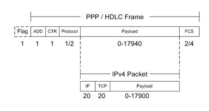
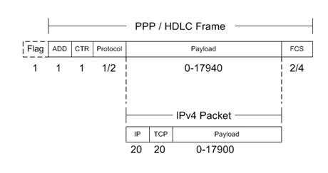
Refer
to Figure 5.1 for a graphic display of the PPP / HDLC header format.
Figure
4.2.1 - PPP / HDLC Framing
PPP
framing is also used widely in dial-up networks. Home access to the Internet was once almost
exclusively dial-up using a standard 64 Kbps channel of which a data modem
could utilize 56 Kbps. Most of these
implementations used PPP encapsulation to wrap the IP packets over the serial
dial-up connection.
5 SONET & POS
Table 7.1 – SONET Common Data rates
|
Interface |
Data Rate |
Without SONET
Overhead |
|
|
|
|
|
OC-3 |
155.52 Mbps |
149.76 Mbps |
|
OC-12 |
622.08 Mbps |
599.04 Mbps |
|
OC-48 |
2.488 Gbps |
2.396 Gbps |
|
OC-192 |
9.953 Gbps |
9.585 Gbps |
|
OC-768 |
39.813 Gbps |
38.339 Gbps |
SONET Rings are deployed all over the world, and
SONET will continue to be a major telecommunications technology using
Fiber-Optics into the foreseeable future.
Most telephone companies have major infrastructure in SONET Rings. The best title I ever saw on a business card
was a reference to SONET networks. The
gentleman managed 17 SONET rings for a major phone company. His title? Ringmaster.
Table 7.1 reflects the optical speeds of SONET
Interfaces. The last column reflects the
payload bandwidth minus the 3.7% overhead required for layer 1 SONET
overhead. SONET overhead is the same
3.7% all the time. It is consistent for
OC-3, OC-12, OC-48, OC-192, and so on. And this reflects the overhead required
for SONET Section, Line, and Path encapsulation of it's
Synchronous Payload Envelopes (SPE) in which data in transferred. So overhead for SONET is easy. It's always 3.7%. This overhead is incurred whenever SONET is
the optical technology being used for transmission (true for ATM over SONET
Optical Interfaces, and Packet over SONET Optical Interfaces).
Packet over SONET
(POS)
RFC
2615 is entitled 'PPP over SONET/SDH', and that is very apropos. But POS interfaces can also support HDLC
encapsulated packets over SONET, and also Frame-Relay encapsulated packets over
SONET. Fortunately, the overhead
associated with each of these encapsulations is identical. The only thing that
varies is the size of the checksum (FCS).
Typically, POS interfaces allow you to choose between a 16 and a 32 bit
checksum (either 2 or 4 bytes trailing the packet and being checked to verify transmission
integrity). The 4 byte header and 1 byte
flag delimiter is the same for PPP, HDLC, and Frame-Relay over SONET. And the engineer chooses to use 2 or 4 byte
FCS sizes.
That
means that, once again, as the overhead is incurred on a per-packet basis, the
smaller the packets, the more of them there are, the more overhead. The bigger the frames, the fewer there are, the less overhead is required to send them. This pretty much holds true for any
technology that supports variable length frames.
Using
the example of the 238 byte IP packet (256 byte IP over Ethernet frame), POS
needs either 245 or 247 bytes to transmit the datagrams
(depending on whether 16 or 32 bits FCS is selected). Often 32 bits checksums are chosen as they
tend to be more accurate. Anyway,
assuming a 32 bit checksum, the average POS overhead ratio would be 96.35%
payload to 3.65% overhead. So POS tends
to be more efficient than ATM or Ethernet for transmitting data packets. And it scales to
much higher speeds than Frame-Relay. If
your main concern is transmitting data traffic, POS is almost always the best
choice. Unless Gigabit
ethernet interfaces cost about the same as an OC-12. Even at its least efficient, a Gigabit
Ethernet interface carries more payload than a POS OC-12. And if the average payload ratio is around
85% payload to 15% overhead for ethernet, then a
Gigabit Ethernet interface will carry about 850 Mbps in payload, which far
exceeds the 600 Mbps an OC-12 is capable of.
6 Layer 3 / 4 Overhead
6.1
IP & IPv6
From
an application layer viewpoint, all lower layer encapsulation is overhead. The overhead is a necessary evil as it is the
packetization and transport of data that facilitates
applications to communicate over wide are networks. But it is still overhead. Most of the technologies that have been
assessed have been viewed from a standpoint of the IP packet is the payload and
the overhead bits are incurred by the physical medium used for transport. But the applications view the IP header and
TCP header as overhead along with the overhead bits incurred by the medium. So it is useful to look at the IP header, the
IPv6 header, UDP and RTP headers, and TCP headers to keep in mind the header
overhead as well as the physical medium overhead as they relate to the upper
applications layers.
Figure
10.1 – IPv4 Header
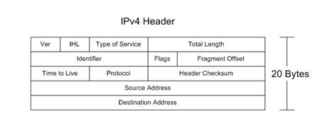
Fields:
Version 4 bits Specifies IP version
Header Length 4 bits Denotes
the Header Length (maximum with option is 60 bytes)
Type of Service 8 bits Field
used for TOS and DiffServ to classify importance (for
Queuing)
Total Length 16 bits Size
of the entire datagram (header + payload)
Identifier 16 bits Used most frequently to identify fragments
Flags 3 bits 1st one is Reserved (must be
zero), 2nd is DF Bit (Don’t Fragment), 3rd is MF Bit
(More Fragments)
Fragment Offset 13 bits Allows
a receiver to determine the place of a fragment in the original unfragmented datagram
Time to Live 8 bits Counts
down from 256 and if it reaches 0, it can indicate a loop, so the packet is
discarded. Orginally
it was meant to count time, but in practice it is a hop count.
Protocol 8 bits Specifies
the Protocol contained in the IP Packet (Usually TCP (6) or UDP (17))
Header Checksum
16 bits This
allows for error checking of the header.
Source Address 32 bits Indicates
the source IP address of the packet (Can be modified by NAT)
Destination Address 32 bits
Indicates the IP address of the recipient host. This field is often the primary field used by
routers to make a forwarding decision for the IP packet.
Note:
There is the ability to lengthen the header with options and padding but the 20
byte header is almost ubiquitous.
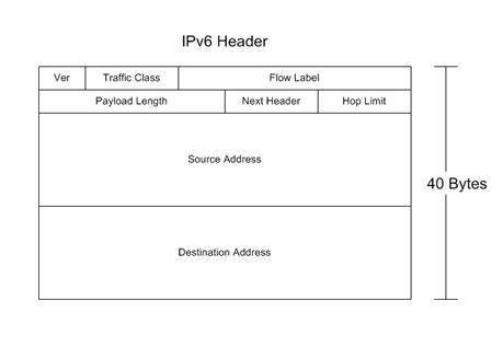
Figure
10.2 – IPv6 Header
6.2
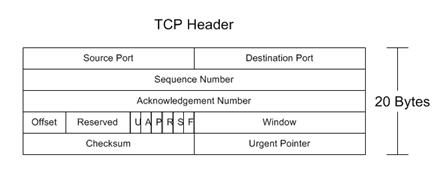
TCP, UDP, & RTP Headers
Figure
10.3 – TCP Header
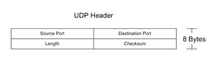
Figure
10.4 – UDP Header
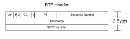
Figure
10.5 – RTP Header
Conclusion
To be fair, the physical layer
technologies covered in this text do a lot more than just carry IP
packets. There are a vast number of
Voice and Video protocols that do not use packetized
IP to communicate. Telecommunications is
more than just the TCP/IP protocol and applications. However, TCP/IP is a large percentage of what
is used by end users and that percentage is growing. So this is not a comprehensive manual on
everything that ATM or Frame-Relay or X.25 does. But it is designed to address how those
protocols interact with IP packets and how IP can be transported over existing
network infrastructures. You could say
this is an IP-centric look at various networking technologies and protocols and
how they are used for transport.
References
IEEE
802.3 Ethernet
Institute of Electrical and
Electronics Engineers. “Carrier
Sense Multiple Access with Collision Detection (CSMA/CD) Access Method and
Physical Layer Specifications”. ISO/IEC
8802-3, IEEE Std. 802.3, 1998.
ATM,
Asynchronous Transfer Mode
Internet Engineering Task
Force. Request for Comments Documents:
RFC 1483 ‘Multiprotocol
Encapsulation over ATM Adaptation Layer 5’, Heinanen,
J., July 1993.
RFC 1626 ‘Default IP MTU
for use over ATM AAL5’, Atkinson, R., May 1994.
RFC 2684 ‘Multiprotocol
Encapsulation over ATM Adaptation Layer 5’, Grossman D., Heinanen,
J., Sept 1999.
Frame-Relay
American National Standards
Institute. Integrated
Services Digital Network (ISDN) – Core Aspects of Frame Protocol for use with
Frame-Relay Bearer Service. ANSI T1.618, 1991.
Frame-Relay Forum
Documents.
FRF.8 (Frame-Relay DLCI to ATM VC Mapping)
International Telecommunications Union Telecommunication
Standardization Sector. ISDN Data Link Specification for Frame Mode Bearer Services. ITU-T Q.922, 1992.
PPP
& HDLC
Internet Engineering Task
Force. Request for Comments Documents:
RFC 1547 ‘Point-to-Point Protocol
Requirements’
RFC 1661 ‘Point-to-Point Protocol’
RFC 1662 ‘PPP in HDLC-like Framing’
SONET
and POS
Internet Engineering Task
Force. Request for Comments Documents:
RFC 1619 ‘PPP over SONET / SDH’
Summary
Have you ever wondered about how IP
packets are transported to and fro across the Internet? What happens to the packets as they traverse
complex physical layer networks using electrical, optical, and wireless
connections? Are you a software
developer interested in knowing more about lower layer network operation and
the implications for application throughput and performance? Are you a network engineer who has one too
many protocol reference posters lining your cubicle but never seem to have the
one you require when you need it? Maybe
you are just trying to understand a bit better how to decode a packet capture
file. What happens to IP packets as they
traverse ATM, Frame-Relay, POS (Packet-over-SONET), 10/100/1000/10G Ethernet,
802.11x Wireless, DSL, DOCSIS (Cable Modem), T1, DS-3, and even Token-Ring,
FDDI, and X.25 networks? Do you just
have a curiosity for knowing why things are the way they are, and understanding
a little about IP packet transport would help in understanding how the Internet
works? If any of these questions
applies, then this book is for you. The
standards and specifications that cover these various technologies would wipe
out a small forest if the documents were actually printed, but this book seeks
to refer to the standards documents and summarize what they say relative to IP
packet overhead, and present it in a clean, easy to use reference text that
will be as useful in 10 years as it is today.
Author Bio